45 how to display data labels in excel chart

› data-analysis › chartsHow to Create Charts in Excel (Easy Tutorial) 1. Select the chart. 2. Click the + button on the right side of the chart, click the arrow next to Legend and click Right. Result: Data Labels. You can use data labels to focus your readers' attention on a single data series or data point. 1. Select the chart. 2. Click a green bar to select the Jun data series. 3. Display every "n" th data label in graphs - Microsoft Community Change the step value (the on in bold) as required Sub PointLabel () Dim mySrs As Series Dim iPts As Long If ActiveChart Is Nothing Then MsgBox "Select a chart and try again.", vbExclamation, "No Chart Selected" Else For Each mySrs In ActiveChart.SeriesCollection With mySrs For iPts = 1 To .Points.count Step 5 ' add label

How To Add Data Labels In Excel - kenh3.info How to Add Data Labels in Excel Excelchat Excelchat from . This method will guide you to manually add a data label from a cell of different column at a time in an excel chart. The mail merge process creates a sheet of mailing labels that you can print, and each label on the sheet contains an address from the list.

How to display data labels in excel chart

How to I rotate data labels on a column chart so that they are ... Then on your right panel, the Format Data Labels panel should be opened. Go to Text Options > Text Box > Text direction > Rotate And the text direction in the labels should be in vertical right now. Hope this information could help you. Regards, Alex Chen * Beware of scammers posting fake support numbers here. Change the format of data labels in a chart To format data labels, select your chart, and then in the Chart Design tab, click Add Chart Element > Data Labels > More Data Label Options. Click Label Options and under Label Contains , pick the options you want. peltiertech.com › excel-column-Column Chart with Primary and Secondary Axes - Peltier Tech Oct 28, 2013 · The second chart shows the plotted data for the X axis (column B) and data for the the two secondary series (blank and secondary, in columns E & F). I’ve added data labels above the bars with the series names, so you can see where the zero-height Blank bars are. The blanks in the first chart align with the bars in the second, and vice versa.

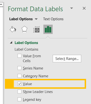
How to display data labels in excel chart. Custom Chart Data Labels In Excel With Formulas - How To Excel At Excel Select the chart label you want to change. In the formula-bar hit = (equals), select the cell reference containing your chart label's data. In this case, the first label is in cell E2. Finally, repeat for all your chart laebls. If you are looking for a way to add custom data labels on your Excel chart, then this blog post is perfect for you. How to Add Data Labels to an Excel 2010 Chart - dummies Use the following steps to add data labels to series in a chart: Click anywhere on the chart that you want to modify. On the Chart Tools Layout tab, click the Data Labels button in the Labels group. A menu of data label placement options... None: The default choice; it means you don't want to ... Excel Charts: Label Last Data Point. Labelling Last Point on an Excel Chart Use the chart wizard to create a line chart based on A1:G9. Select the 4th data series 'Label Last 1' and format series to have border and marker None. Also enabled Data Label Value. Repeat for 5th and 6th data series. Format the plot area as required. Here I have removed the border, major gridlines and changed the plot area color. Data Labels in Excel Pivot Chart (Detailed Analysis) Click on the Plus sign right next to the Chart, then from the Data labels, click on the More Options. After that, in the Format Data Labels, click on the Value From Cells. And click on the Select Range. In the next step, select the range of cells B5:B11. Click OK after this.

Display Data Labels Above Data Markers in Excel Chart We use the following steps: Right-click one of the blue data markers. The chart is activated, and all the data markers are selected. Click Add Data Labels on the shortcut menu and choose Add Data Labels on the flyout menu. support.microsoft.com › en-us › officeAdd or remove data labels in a chart - support.microsoft.com Click the data series or chart. To label one data point, after clicking the series, click that data point. In the upper right corner, next to the chart, click Add Chart Element > Data Labels. To change the location, click the arrow, and choose an option. If you want to show your data label inside a text bubble shape, click Data Callout. How To Add Data Labels In Excel - fuhou.info By Vaseline. How To Add Data Labels In Excel. Right click the data series in the chart, and select add data labels > add. In this case, the first label is in cell e2. This method will guide you to manually add a data label from a cell of different column at a time in an excel chart. The mail merge process creates a sheet of mailing labels that ... How to use data labels in a chart - YouTube Excel charts have a flexible system to display values called "data labels". Data labels are a classic example a "simple" Excel feature with a huge range of o...

› charts › gauge-templateExcel Gauge Chart Template - Free Download - How to Create Labels: These determine the intervals of the gauge chart labels. Levels: These are the value ranges that will split the dial chart into multiple sections. The more detailed you want to display your data, the more value intervals you’ll need. Pointer: This determines the width of the needle (the pointer). You can change the width however you ... How to Add Two Data Labels in Excel Chart (with Easy Steps) 4 Quick Steps to Add Two Data Labels in Excel Chart. Step 1: Create a Chart to Represent Data. Step 2: Add 1st Data Label in Excel Chart. Step 3: Apply 2nd Data Label in Excel Chart. Step 4: Format Data Labels to Show Two Data Labels. Things to Remember. Add a DATA LABEL to ONE POINT on a chart in Excel All the data points will be highlighted. Click again on the single point that you want to add a data label to. Right-click and select ' Add data label '. This is the key step! Right-click again on the data point itself (not the label) and select ' Format data label '. You can now configure the label as required — select the content of ... Adding rich data labels to charts in Excel 2013 Putting a data label into a shape can add another type of visual emphasis. To add a data label in a shape, select the data point of interest, then right-click it to pull up the context menu. Click Add Data Label, then click Add Data Callout . The result is that your data label will appear in a graphical callout.

Directly Labeling Excel Charts - PolicyViz

Excel charts: how to move data labels to legend Click anywhere on the chart. On the Design tab of the ribbon (under Chart Tools), in the Chart Layouts group, click Add Chart Element > Data Table > With Legend Keys (or No Legend Keys if you prefer) 0 Likes

Aligning data point labels inside bars | How-To | Data ...

peltiertech.com › excel-column-Column Chart with Primary and Secondary Axes - Peltier Tech Oct 28, 2013 · The second chart shows the plotted data for the X axis (column B) and data for the the two secondary series (blank and secondary, in columns E & F). I’ve added data labels above the bars with the series names, so you can see where the zero-height Blank bars are. The blanks in the first chart align with the bars in the second, and vice versa.

How to Add Data Labels in Excel - Excelchat | Excelchat

Change the format of data labels in a chart To format data labels, select your chart, and then in the Chart Design tab, click Add Chart Element > Data Labels > More Data Label Options. Click Label Options and under Label Contains , pick the options you want.

How to Use Cell Values for Excel Chart Labels

How to I rotate data labels on a column chart so that they are ... Then on your right panel, the Format Data Labels panel should be opened. Go to Text Options > Text Box > Text direction > Rotate And the text direction in the labels should be in vertical right now. Hope this information could help you. Regards, Alex Chen * Beware of scammers posting fake support numbers here.

How to add or move data labels in Excel chart?

How to suppress 0 values in an Excel chart | TechRepublic

How to Add Data Labels to your Excel Chart in Excel 2013

Excel Charts: Dynamic Label positioning of line series

Add or remove data labels in a chart

Change the format of data labels in a chart

Add Labels ON Your Bars

Adding rich data labels to charts in Excel 2013 | Microsoft ...

data visualization - How do you put values over a simple bar ...

Bar charts with long category labels; Issue #428 November 27 ...

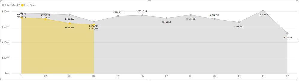
How to add live total labels to graphs and charts in Excel ...

Is there a way to show different data labels in a bar chart ...

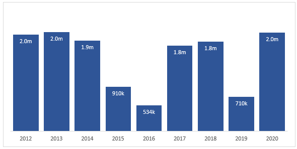
Dynamic Number Format for Millions and Thousands - PK: An ...

Enable or Disable Excel Data Labels at the click of a button ...

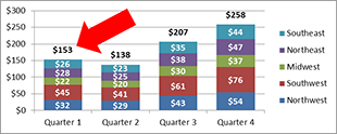
How to Add Totals to Stacked Charts for Readability - Excel ...

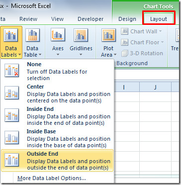
Excel 2010: Show Data Labels In Chart

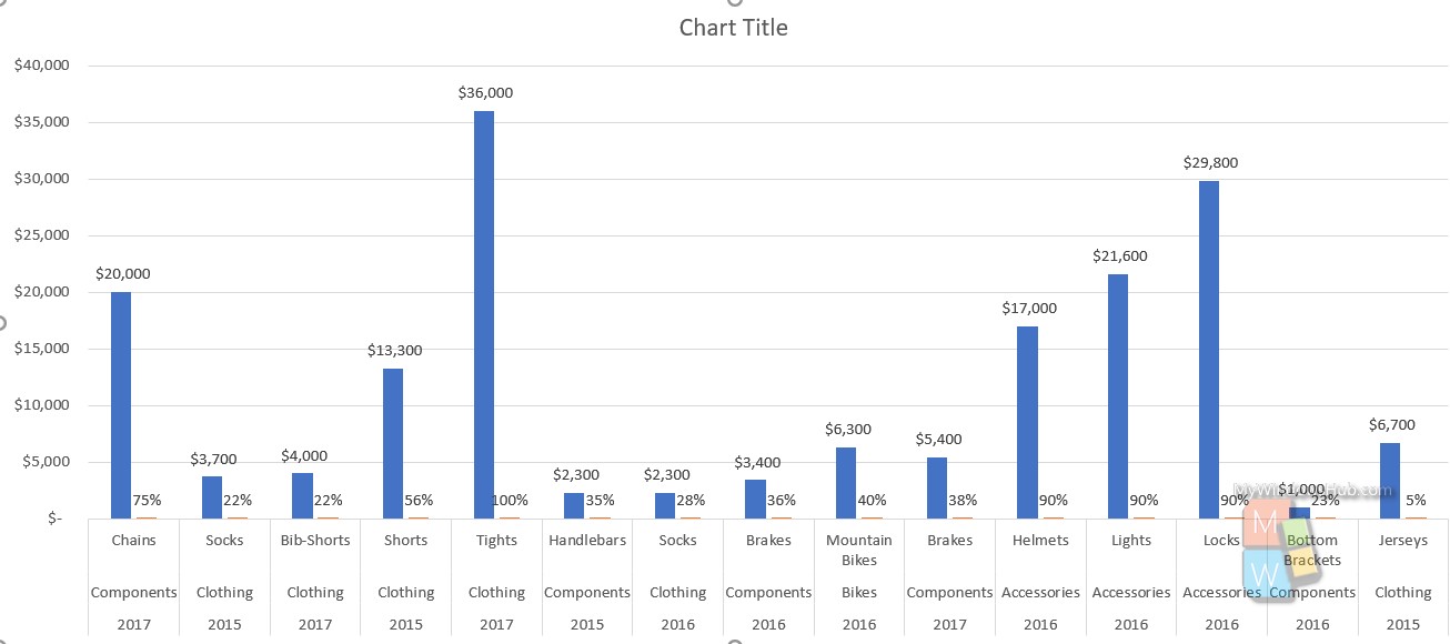
Fixed:] Excel Chart Is Not Showing All Data Labels (2 Solutions)

Solved: How to show all detailed data labels of pie chart ...

Adding rich data labels to charts in Excel 2013 | Microsoft ...

How To Show Or Hide Data Labels On MS Excel? | My Windows Hub

microsoft excel - Adding data label only to the last value ...

Solved: Area chart data labels not in correct positions ...

Add Total Values for Stacked Column and Stacked Bar Charts in ...

Format Number Options for Chart Data Labels in PowerPoint ...

How-to Use Data Labels from a Range in an Excel Chart - Excel ...

How to add data labels from different column in an Excel chart?

Adding Data Labels to Your Chart (Microsoft Excel)

How to Get Colors in Excel Chart Data Lables - Formatting Trick

How to Add Axis Labels to a Chart in Excel | CustomGuide

Show Trend Arrows in Excel Chart Data Labels

Format Chart Numbers as Thousands or Millions — Excel ...

how to add data labels into Excel graphs — storytelling with data

How to Show Percentages in Stacked Column Chart in Excel ...

Change Horizontal Axis Values in Excel 2016 - AbsentData

Directly Labeling Excel Charts - PolicyViz

Directly Labeling Your Line Graphs | Depict Data Studio

Excel charts: add title, customize chart axis, legend and ...

Excel charts: add title, customize chart axis, legend and ...

Solved: How to show all detailed data labels of pie chart ...

Custom data labels in a chart

Change the format of data labels in a chart

Share :