44 excel pivot table repeat item labels disabled
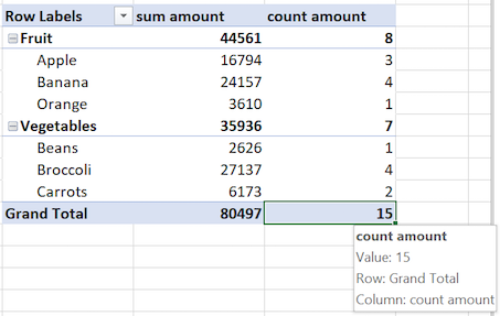
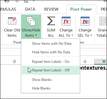
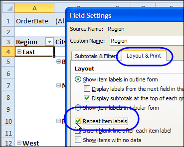
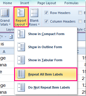
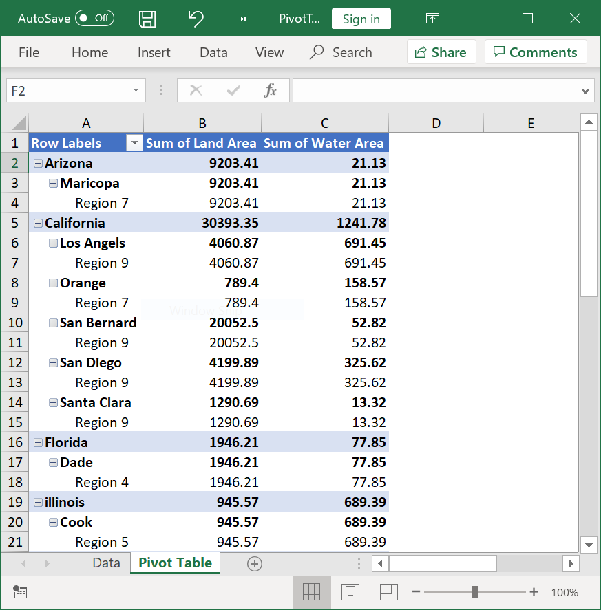
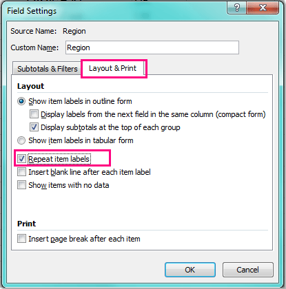
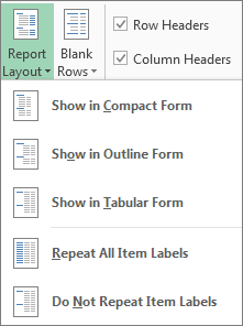
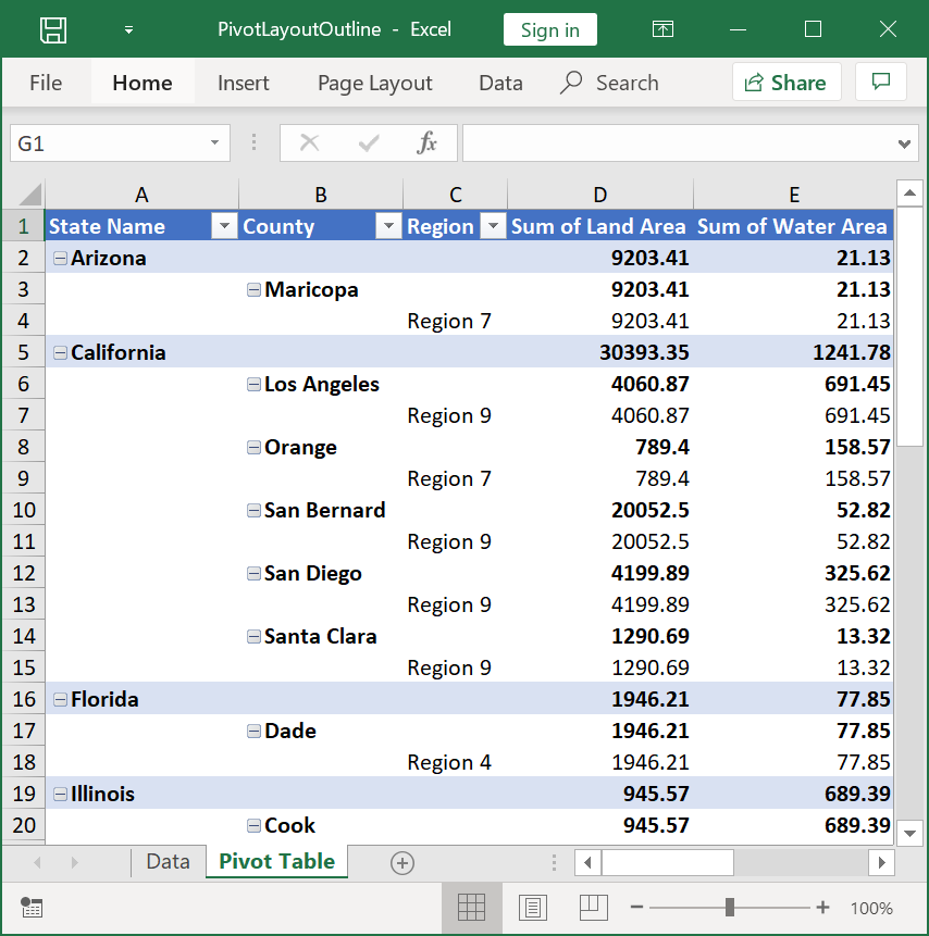
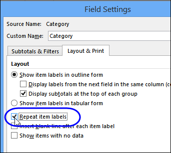
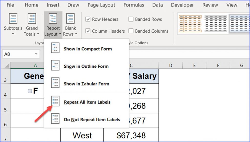
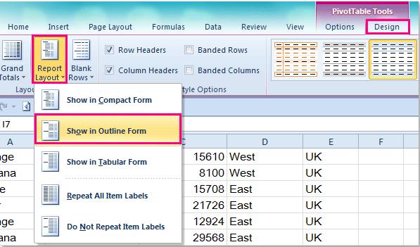
How to Group Data in Pivot Table (3 Simple Methods) Steps: At the very beginning, select the dataset and insert a PivotTable. Next, make sure to select the New Worksheet option and press OK. Then, group the data by going to the PivotTable Analyze tab and selecting Group Selection. In turn, the various groups appear as shown in the picture below. Excel Pivot Tables - Page 23 - by contextures.com Repeat the Row Labels. A new feature in Excel 2010 lets you repeat those row labels, so they appear on every row in the pivot table. To turn on that feature for all the fields, select the Repeat All Item Labels on the Ribbon's Design tab. Here's the pivot table in Outline form, with repeating row labels. Repeating Labels for a Single Field
Microsoft Excel - Pivot Tables | Nicholls State University Microsoft Excel - Pivot Tables. Maximize your investment in Microsoft Excel by mastering its pivot table features. In this practical hands-on course, you will discover how to use different layout, subtotaling, and filtering options and discover a variety of advanced techniques for pivot tables, including Pivot Charts, Timelines, and Slicers.
Excel pivot table repeat item labels disabled
Excel Pivot Table Subtotals Examples Videos Workbooks Right-click a label for the field in which you want to change the subtotal. In this example, right-click cell B5, which has the Install label. In the pop-up menu, click Field Settings. In the Field Settings dialog box, click the Subtotals & Filters tab. Under Subtotals, click Custom. [Fixed] Excel Pivot Table: Cannot Group That Selection (2 ... - ExcelDemy I will use the following Product Order Record as a dataset to demonstrate all the solutions. In the dataset, I've different product names with their amount and country. I also have all the products' corresponding Order Date and Ship Date.. I will try to group all the Ship Dates.But look, the Ship Date column has a mix of various date formats as well as invalid dates. Resolving Duplicate Values Within Excel Pivot Tables Activate Excel's Data menu. Click Text to Columns. In the Text to Column Wizard simply click Finish, in this context you don't need to make any choices or work through the steps. Right-click any cell within the pivottable. Choose the Refresh command. Notice that now the duplicate amounts for account 4000 are consolidated into a single value.
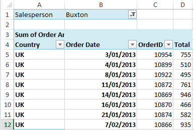
Excel pivot table repeat item labels disabled. excel - Select pivot item - Stack Overflow hi, thank you for the fast answer. The problem is that I do not know the range, I do not know how many elements the Pivot Table has. So, my plan is to go through each item of a particular column of the pivot table. But how do i select/activate each cell while looping? pivotfields.PivotItems.select does not work. thank you! - Ranking values in Pivot Table with multiple row labels Hoping someone can help. Thanks! I have a pivot table with multiple Row Labels: Player and Team. I then have a bunch of stat categories under Values, one of which is 'Pts'. I have the table sorted by Pts, but I need a 'Ranking' column. I created a second Pts column and used 'Show Values As - Rank Largest to Smallest', but it's not working. How to Create a Pivot Table in Excel: Step-by-Step - CareerFoundry As a first step, you should select the entire table (you can easily do this by using the keyboard shortcut (starting from cell A2) Ctrl+Shft+right arrow+down arrow for Windows or Cmd+Shft+right arrow+down arrow for Mac). Once the entire table is selected, go to the ribbon above in your Excel and click on the Insert tab. [Fixed] Excel Pivot Table Not Grouping Dates by Month - ExcelDemy Next, use this table to create the Pivot Table. If you need to see how to create a Pivot Table then go to Section 1. Also, follow the procedure of Section 1 to insert dates and sales into the respective fields of the Pivot Table. Later, you will see your Pivot Table carries the Sales information by Month.
Pivot table enhancements - EPPlus Software EPPlus 5.4 adds support for pivot table filters, calculated columns and shared pivot table caches. The following filters are supported. Item filters - Filters on individual items in row/column or page fields. Caption filters (label filters) - Filters for text on row and column fields. Date, numeric and string filters - Filters using various ... Pivot Table Grouping, Ungrouping And Conditional Formatting So let's drag the Age under the Rows area to create our Pivot table. #1) Right-click on any number in the pivot table. #2) On the context menu, click Group. #3) Grouping dialog box appears, in this example, the least number is 25, so by default the Starting number is entered as 25, and you can change if necessary. What Is An Excel Pivot Table And How To Create One - Software Testing Help It is a data analysis tool with many user-friendly features. Excel allows you to use the data source present in the excel or any external files and build the Pivot table from the Insert -> PivotTable option. You can then build your desired table using fields, sort, group, settings, etc. feature available in the PivotTable Analyse ribbon. ayesdeeef/Microsoft-Excel---Data-Analysis-with-Excel-Pivot-Tables Microsoft-Excel---Data-Analysis-with-Excel-Pivot-Tables. This portfolio contains my homework assignments for the Udemy course on Pivot Tables in Microsoft Excel by Chris, the Founder of Maven Analytics. I have completed these assignments entirely by myself without the assistance of others and without looking at any solutions available online.
How to Create a Pivot Table in Excel? - Great Learning Here is the Step By Step Guide to creating a pivot table. Step1: In Excel for Windows, make a PivotTable. Choose the cells from which you want to create a PivotTable. Go to Insert Option and click on Pivot Table. Select the location for the PivotTable report. At last, click on the OK option. Excel Pivot Tables: Using Slicers to Filter Data To use the slicer, simply click on the items that you want to include in your pivot table. For example, if you only want to see data for the states of "CA" only, click on "CA". The pivot table will update to only include data for that state. And if you want to filter and include bot, hold Shift and click both "CA" and "NY". How to make and use Pivot Table in Excel - Ablebits.com 2. Create a Pivot Table. Select any cell in the source data table, and then go to the Insert tab > Tables group > PivotTable. This will open the Create PivotTable window. Make sure the correct table or range of cells is highlighted in the Table/Range field. Then choose the target location for your Excel Pivot Table: Pivot Table formatting after refresh - Page 2 - Microsoft Community Hub Pivot Table formatting after refresh. I have a pivot table set up, and have selected "Preserve cell formatting on update" in PivotTable Option. However, when I select a different slicer or refresh the data, the cell formats change dramatically and seemingly randomly. I cannot get the table to save the cell format consistently.
How to use Pivot Tables – Excel's most powerful feature and ...
A Pivotchart Pivot Table Excel Labels - Otosection Surface Studio vs iMac - Which Should You Pick? 5 Ways to Connect Wireless Headphones to TV. Design

Repeat Pivot Table row labels • AuditExcel.co.za Pivot Tables ...
Table.Pivot - PowerQuery M | Microsoft Learn Table.Pivot(table as table, pivotValues as list, attributeColumn as text, valueColumn as text, optional aggregationFunction as nullable function) as table About. Given a pair of columns representing attribute-value pairs, rotates the data in the attribute column into a column headings.
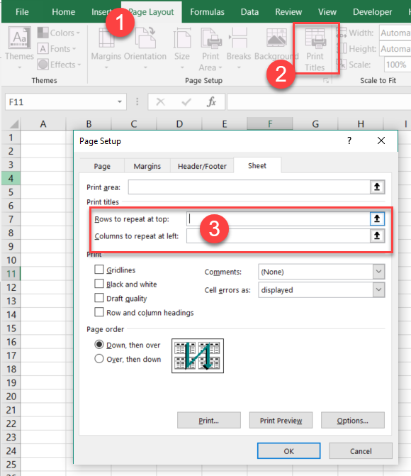
Excel 2016 in Windows10. Can't use "rows to repeat at top ...
Resolving Duplicate Values Within Excel Pivot Tables Activate Excel's Data menu. Click Text to Columns. In the Text to Column Wizard simply click Finish, in this context you don't need to make any choices or work through the steps. Right-click any cell within the pivottable. Choose the Refresh command. Notice that now the duplicate amounts for account 4000 are consolidated into a single value.
Pivot Table Settings | Documents for Excel .NET Edition ...
[Fixed] Excel Pivot Table: Cannot Group That Selection (2 ... - ExcelDemy I will use the following Product Order Record as a dataset to demonstrate all the solutions. In the dataset, I've different product names with their amount and country. I also have all the products' corresponding Order Date and Ship Date.. I will try to group all the Ship Dates.But look, the Ship Date column has a mix of various date formats as well as invalid dates.

Get rid of the GETPIVOTDATA without disabling it | wmfexcel
Excel Pivot Table Subtotals Examples Videos Workbooks Right-click a label for the field in which you want to change the subtotal. In this example, right-click cell B5, which has the Install label. In the pop-up menu, click Field Settings. In the Field Settings dialog box, click the Subtotals & Filters tab. Under Subtotals, click Custom.

Top 25 Advanced Pivot Table Tips and Tricks
Formatting Tips for Pivot Tables - Goodly
Pivot Table Settings | Documents for Excel .NET Edition ...
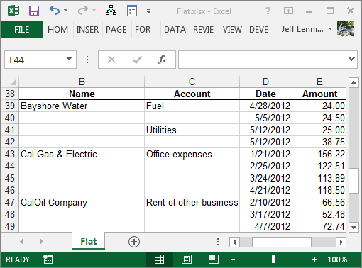
How to Flatten Data in Excel Pivot Table? - GeeksforGeeks
Turn Repeating Item Labels On and Off | Excel Pivot Tables

Turn off automatic date and time grouping in Excel Pivot Tables
Repeat All Item Labels In An Excel Pivot Table | MyExcelOnline
Excel Pivot Tables to Extract Data • My Online Training Hub

4 Excel Settings - Xelplus - Leila Gharani
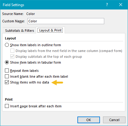
Pivot Table: Pivot table display items with no data | Exceljet
PIvot Tables: "Show items in tabular form" & "Repeat Item ...

Excel Pivot Table Report Layout

Get rid of the GETPIVOTDATA without disabling it | wmfexcel

Fix Excel Pivot Table Missing Data Field Settings
Repeat Pivot Table Labels in Excel 2010 | Excel Pivot Tables

Oracle Enterprise Performance Management Workspace, Fusion ...

Working with Pivot Tables | Excel library | Syncfusion

Everything analysts need to know about pivot tables
How to repeat row labels for group in pivot table?

Solved: Repeat Row Labels(Headers) in Metrics - Microsoft ...

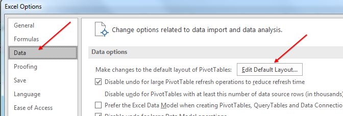
Set PivotTable default layout options
Working with Pivot Tables | Excel library | Syncfusion
How to repeat row labels for group in pivot table?
Set Defaults For All Future Pivot Tables - Excel Tips ...

Pivot Table Tutorial (100 Tips and Tricks) | Basic to Advanced
Repeat item labels in a PivotTable
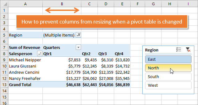
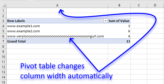
How to Stop Pivot Table Columns from Resizing on Change or ...

Repeat Pivot Table row labels • AuditExcel.co.za Pivot Tables ...
Working with Pivot Tables | Excel library | Syncfusion
Turn Repeating Item Labels On and Off | Excel Pivot Tables
Repeating Values in Pivot Tables – Daily Dose of Excel
How to Repeat Item Labels in Pivot Table - ExcelNotes
Excel Pivot Tables - Sorting Data
Repeat All Item Labels In An Excel Pivot Table | MyExcelOnline
Excel Pivot Tables Explained • My Online Training Hub
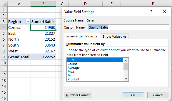
How to Use Pivot Table Field Settings and Value Field Setting

Excel Pivot Table Group: Step-By-Step Tutorial To Group Or ...
How to repeat row labels for group in pivot table?

Pivot Table Tutorial (100 Tips and Tricks) | Basic to Advanced
Post a Comment for "44 excel pivot table repeat item labels disabled"