41 conditional formatting pivot table row labels

Sunburst Chart in Excel - Example and Explanations This column will be used to define the size of the segments. Select one of the cells in your data table. Go to the menu Insert> Hierarchical graph> Sunburst. Immediately, the sunbeams graph appears on your worksheet. Tips and tricks for formatting in reports - Power BI | Microsoft Docs Open the Formatting pane by selecting the paint roller icon and then choose the Data colors card. Next to Default color, select the fx icon. In the Default color pane, use the dropdowns to identify the fields to use for conditional formatting.

Control row & column headings in a paginated report - Microsoft Report ... In a table or matrix, the first row usually contains column headings that label data in each column; the first column usually contains row headings that label the data in each row. For nested groups, you might want to repeat the initial set of row and column headings that contain group labels. By default, a list data region does not include ...

Conditional formatting pivot table row labels

Excel Pivot Table Macro Paste Format Values Follow these steps to copy a pivot table's values and formatting: Select the original pivot table, and copy it. Click the cell where you want to paste the copy. On the Excel Ribbon's Home tab, click the Dialog Launcher button in the Clipboard group . In the Clipboard, click on the pivot table copy, in the list of copied items.. Pivot Keeps Table Changing Formatting the easiest way is to just turn on the macro recorder and apply the conditional formatting manually home > conditional formatting > clear rules > clear rules from selected cells pivot table formatting keeps changing in the simplest pivot table, one identifies a row value, a column value, and a data value usually they think they are helping and … How to change cell formatting using a Drop Down list Select cell D3. Go to tab "Data" on the ribbon. Press with left mouse button on "Data Validation" button on the ribbon and a dialog box appears. Go to tab "Settings" on the dialog box. See image below. Select List. Type: No formatting, %, Time, Above Average, Below Average.

Conditional formatting pivot table row labels. How to use Conditional Formatting in Excel to Color-Code Specific Cells ... 3. Choose Conditional Formatting from the ribbon. 5. We're going to color-code bills that we haven't paid. To do that, add "NO" to the Format cells that are EQUAL TO box, and then select a color... Conditional formatting for a text column - Power BI Go to the field, use the drop down in the fields section and choose ' conditional formatting ' - choose Background or Font colour. Choose ' Rules ' for ' Format by '. ' Summarization ' as ' Minimum '. Choose the number and the colour I f value is '1' then 'Green'. Click OK and it should work 🙂. How to Use Excel Pivot Table Label Filters Right-click a cell in the pivot table, and click PivotTable Options. In the PivotTable Options dialog box, click the Totals & Filters tab In the Filters section, add a check mark to 'Allow multiple filters per field.' Click the OK button, to apply the setting and close the dialog box. Quick Way to Hide or Show Pivot Items Excel conditional formatting based on another cell text [5 ways] Click on the Format option to open the Format Cells dialogue box. In the Format Cells dialogue box under the Fill option, select the color you want and press OK. After this, you can see the color you choose in the Preview option. Now press OK in the New Formatting Rule dialogue box to apply the formatting. You will get the below result after this.

Conditional Formatting in JavaScript Pivot Table control To do so, open the conditional formatting dialog and edit the "Value", "Condition" and "Format" options based on user requirement and click "OK". To remove a conditional format, click the "Delete" icon besides the respective condition. Event ConditionalFormatting Create a matrix visual in Power BI - Power BI | Microsoft Docs When you turn on Row subtotals and add a label, Power BI also adds a row, and the same label, for the grand total value. ... For more information, see Conditional table formatting. Shading and font colors with matrix visuals. With the matrix visual, you can apply conditional formatting (colors and shading and data bars) to the background of ... Formatting Pivot Table Keeps Changing Search: Pivot Table Formatting Keeps Changing. We then try to find our own method - copy paste the pivot table as values and then do the calculations Both; Neither; The Answer is D as a Pivot Table can be used to create a Pivot Chart and a Pivot Table can be created on an Existing sheet In the PivotTable Options dialog box, click Layout & Format tab, and then check As a consequence if you ... Solved: Conditional Formatting for Dates - Power BI The last step is to select the conditional formatting for the Original Submittal Date, selected Format by Rules, based on field Past Due/Within 7 Days Submittal, and if the number was 1 I chose a red format, if the value was 2 I chose a yellow format. And that did it! Thank you both, @amitchandak and @Bizualisation View solution in original post

Add filter option for all your columns in a pivot table Now, I'm trying to figure out how to see the value filter just below the Number filters in the right-click menu, and I dont see in it my Pivot. I have downloaded a sample excel with a pivot which already has the value filter. I'm trying to create my own pivot in this sample excel using the same data set, but I just dont see the value filer. Excel Pivot Table Conditional Formatting Row Labels Go making the conditional formatting select the color scale and do it based on commercial and choose diverging and the colors should give expected result. Here a glaze color or bar and been applied... Changing Pivot Table Keeps Formatting Here's how you can do it However, if you change the Pivot Table row/column fields then the conditional formatting will be lost Select the Formatting tab (if not already selected) At the top of Excel, click the File tab As a consequence if you add a new column to the tabel you have to As a consequence if you add a new column to the tabel you ... In a pivot table, how to apply conditional formatting by label instead ... In a pivot table you can apply a conditional formatting to a group of value rather than to a cell or to the whole field thank to the "Applies to" option of the "Edit rule" window. My objective here is to make the fill colour change at thresholds that are different for each item rows.

Pivot Table Row Labels In the Same Line - Beat Excel!

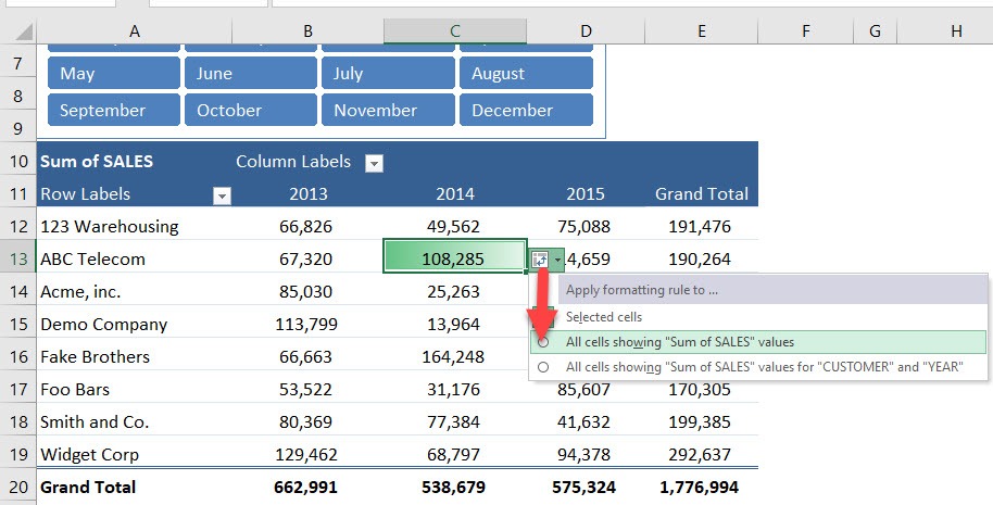
How to Show Text in Pivot Table Values Area - Contextures Excel Tips On the Excel Ribbon's Home tab, click Conditional Formatting Then click New Rule, to open the New Formatting Rule dialog box In the Apply Rule to section, select the 3rd option - All cells showing 'Max of RegID' values for 'City' and 'Store'. This option creates flexible conditional formatting that will adjust if the pivot table layout changes.

How to Create a MS Excel Pivot Table – An Introduc

Apply conditional table formatting in Power BI - Power BI To apply conditional formatting, select a Table or Matrix visualization in Power BI Desktop. In the Visualizations pane, right-click or select the down-arrow next to the field in the Values well that you want to format. Select Conditional formatting, and then select the type of formatting to apply. Note

Conditionally Format a Pivot Table With Data Bars | MyExcelOnline

Excel Pivot Table Report Filter Tips and Tricks To show the Report Filters across the row: Right-click a cell in the pivot table, and click Pivot Table Options On the Layout & Format tab, click the drop down arrow beside 'Display Fields in Report Filter Area' Click 'Over, Then Down' In the 'Report filter fields per row' box, select the number of filters to go across each row.

Accelerate Your Analysis with Pivot Table | Simplified Excel

EXTENDED LEARNING MODULE D (Web Version) Power Point • Basic Filter supports only "equal to" criteria • Example: customers in the North REGION Basic Filter Steps 1. Open workbook (XLMD_Customer.xls from ) 2. Click in any cell in the list 3. Menu bar - click on Data and then click on Filter • Will see list box arrows next to each label or column heading Basic Filter Steps

March 2012 | OPTION EXPLICIT VBA

Y/N I can use conditional cell formatting to visually represen steps and go right to conditional cell formatting. 1. In a new Excel workbook, enter the numbers 1 to 12 in cells A1 to A12. Mouse over the column of cells to select it. To the lower right of cell A12 you should see the Quick Analysis icon. Click on the icon.

How to repeat row labels for group in pivot table?

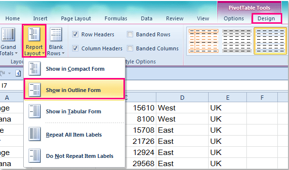
How to Format Excel Pivot Table - Contextures Excel Tips Follow these steps to copy a pivot table's values and formatting: Select the original pivot table, and copy it. Click the cell where you want to paste the copy. On the Excel Ribbon's Home tab, click the Dialog Launcher button in the Clipboard group . In the Clipboard, click on the pivot table copy, in the list of copied items..

Share :