43 excel scatter chart labels

How To Create Scatter Chart in Excel? - EDUCBA To apply the scatter chart by using the above figure, follow the below-mentioned steps as follows. Step 1 - First, select the X and Y columns as shown below. Step 2 - Go to the Insert menu and select the Scatter Chart. Step 3 - Click on the down arrow so that we will get the list of scatter chart list which is shown below. Creating Scatter Plot with Marker Labels - Microsoft Community Right click any data point and click 'Add data labels and Excel will pick one of the columns you used to create the chart. Right click one of these data labels and click 'Format data labels' and in the context menu that pops up select 'Value from cells' and select the column of names and click OK.

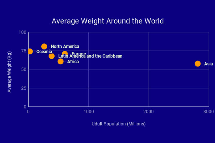
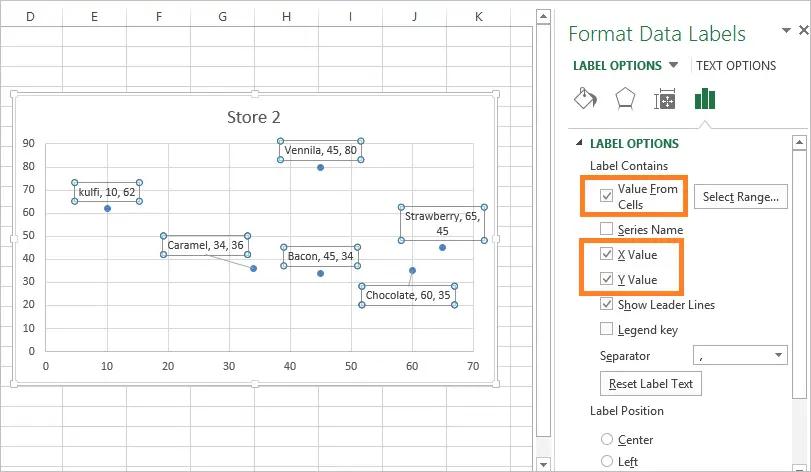
How to find, highlight and label a data point in Excel scatter plot Select the Data Labels box and choose where to position the label. By default, Excel shows one numeric value for the label, y value in our case. To display both x and y values, right-click the label, click Format Data Labels…, select the X Value and Y value boxes, and set the Separator of your choosing: Label the data point by name

Excel scatter chart labels

› excel-chart-verticalExcel Chart Vertical Axis Text Labels - My Online Training Hub Apr 14, 2015 · Note how the vertical axis has 0 to 5, this is because I've used these values to map to the text axis labels as you can see in the Excel workbook if you've downloaded it. Step 2: Sneaky Bar Chart. Now comes the Sneaky Bar Chart; we know that a bar chart has text labels on the vertical axis like this: How do I set labels for each point of a scatter chart? Answer trip_to_tokyo Volunteer Moderator | Article Author Replied on September 14, 2011 Click one of the data points on the chart. Chart Tools. Layout contextual tab. Labels group. Click on the drop down arrow to the right of:- Data Labels Make your choice. If my comments have helped please vote as helpful. Thanks. Report abuse How to Add Labels to Scatterplot Points in Excel - Statology Step 3: Add Labels to Points. Next, click anywhere on the chart until a green plus (+) sign appears in the top right corner. Then click Data Labels, then click More Options…. In the Format Data Labels window that appears on the right of the screen, uncheck the box next to Y Value and check the box next to Value From Cells.

Excel scatter chart labels. support.microsoft.com › en-us › topicPresent your data in a scatter chart or a line chart Scatter charts and line charts look very similar, especially when a scatter chart is displayed with connecting lines. However, the way each of these chart types plots data along the horizontal axis (also known as the x-axis) and the vertical axis (also known as the y-axis) is very different. Improve your X Y Scatter Chart with custom data labels Select the x y scatter chart. Press Alt+F8 to view a list of macros available. Select "AddDataLabels". Press with left mouse button on "Run" button. Select the custom data labels you want to assign to your chart. Make sure you select as many cells as there are data points in your chart. Press with left mouse button on OK button. Back to top [Solved] Excel Scatter Chart with Labels | 9to5DevOps Doesn't work though. This works if and only if the numbers in column 'B' are whole numbers. The excel chart isn't really using any of the data in column B anymore. The only way I have been able to reliably do this in the past is to make every row of data it's own data series. Painful, but if you want to see it in action, I have an example excel ... Add or remove data labels in a chart - support.microsoft.com Click the data series or chart. To label one data point, after clicking the series, click that data point. In the upper right corner, next to the chart, click Add Chart Element > Data Labels. To change the location, click the arrow, and choose an option. If you want to show your data label inside a text bubble shape, click Data Callout.

Excel scatter chart using text name - Access-Excel.Tips Since Excel allows different chart types to be displayed in one chart, we are going to create a mix of bar chart (column chart) and scatter chart. Scatter chart is used to display the actual data point, while bar chart is to display Grade labels. - Create scatter chart for Range B20:C31 (Series 1) Create an X Y Scatter Chart with Data Labels - YouTube How to create an X Y Scatter Chart with Data Label. There isn't a function to do it explicitly in Excel, but it can be done with a macro. The Microsoft Kno... How to create a scatter plot and customize data labels in Excel During Consulting Projects you will want to use a scatter plot to show potential options. Customizing data labels is not easy so today I will show you how th... How to add axis label to chart in Excel? - ExtendOffice Navigate to Chart Tools Layout tab, and then click Axis Titles, see screenshot: 3.

How to Find, Highlight, and Label a Data Point in Excel Scatter Plot? By default, the data labels are the y-coordinates. Step 3: Right-click on any of the data labels. A drop-down appears. Click on the Format Data Labels… option. Step 4: Format Data Labels dialogue box appears. Under the Label Options, check the box Value from Cells . Step 5: Data Label Range dialogue-box appears. peltiertech.com › multiple-time-series-excel-chartMultiple Time Series in an Excel Chart - Peltier Tech Aug 12, 2016 · This discussion mostly concerns Excel Line Charts with Date Axis formatting. Date Axis formatting is available for the X axis (the independent variable axis) in Excel’s Line, Area, Column, and Bar charts; for all of these charts except the Bar chart, the X axis is the horizontal axis, but in Bar charts the X axis is the vertical axis. Labeling X-Y Scatter Plots (Microsoft Excel) Just enter "Age" (including the quotation marks) for the Custom format for the cell. Then format the chart to display the label for X or Y value. When you do this, the X-axis values of the chart will probably all changed to whatever the format name is (i.e., Age). Scatter chart horizontal axis labels | MrExcel Message Board If you must use a XY Chart, you will have to simulate the effect. Add a dummy series which will have all y values as zero. Then, add data labels for this new series with the desired labels. Locate the data labels below the data points, hide the default x axis labels, and format the dummy series to have no line and no marker. oereich said: Hi,

Add Custom Labels to x-y Scatter plot in Excel - DataScience Made Simple

Scatter Plots in Excel with Data Labels To add the lines between points "C" and "D" select any of them then right click on the mouse and choose "Change Series Chart Type" select then "C" and "D" and change them to "Scatter with straight ...

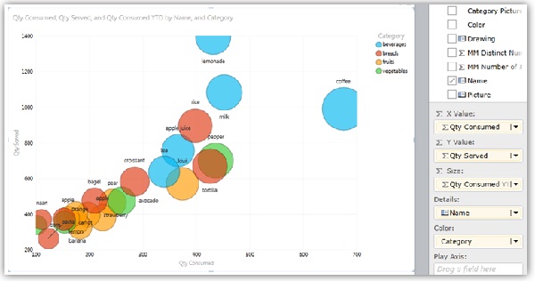
Bubble and scatter charts in Power View - Excel

How do I get a label in a scatter plot instead of "Series 1 Point"? They are not actually labels, by the way. They show series name, point number (the X value), and the X and Y values in parentheses. Yeah, X appears twice. In order to see the location, you need to set up the chart to have one series per row of the data. Tedious by hand, though possible. Easier with VBA.

Google Sheets - Add Labels to Data Points in Scatter Chart

Hover labels on scatterplot points - Excel Help Forum You can not edit the content of chart hover labels. The information they show is directly related to the underlying chart data, series name/Point/x/y You can use code to capture events of the chart and display your own information via a textbox. Cheers Andy Register To Reply

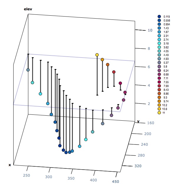
3d scatter plot for MS Excel

How To Add Axis Labels In Excel [Step-By-Step Tutorial] First off, you have to click the chart and click the plus (+) icon on the upper-right side. Then, check the tickbox for 'Axis Titles'. If you would only like to add a title/label for one axis (horizontal or vertical), click the right arrow beside 'Axis Titles' and select which axis you would like to add a title/label.

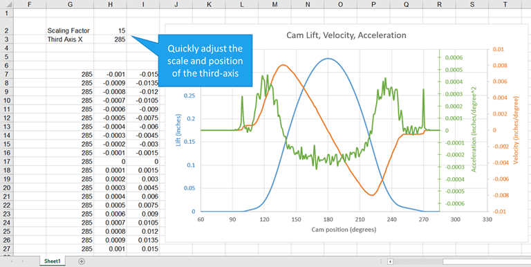
How to Add a Third Y-Axis to a Scatter Chart | EngineerExcel

› add-vertical-line-excel-chartAdd vertical line to Excel chart: scatter plot, bar and line ... May 15, 2019 · Add vertical line to Excel scatter chart; Insert vertical line in Excel bar chart; Add vertical line to line chart; How to add vertical line to scatter plot. To highlight an important data point in a scatter chart and clearly define its position on the x-axis (or both x and y axes), you can create a vertical line for that specific data point ...

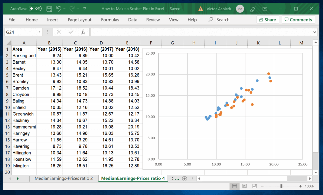
How to Make a Scatter Plot in Excel | Itechguides.com

support.microsoft.com › en-us › topicHow to use a macro to add labels to data points in an xy ... The labels and values must be laid out in exactly the format described in this article. (The upper-left cell does not have to be cell A1.) To attach text labels to data points in an xy (scatter) chart, follow these steps: On the worksheet that contains the sample data, select the cell range B1:C6.

Add Custom Labels to x-y Scatter plot in Excel - DataScience Made Simple

Excel: labels on a scatter chart, read from array - Stack Overflow Excel: labels on a scatter chart, read from array Ask Question 0 Here I have a chart I did a right-click -> "Add labels" , and it read them from my a (H/C) row. Basically, I want it to read label values from the CO2/CH4 row instead, so they would be 0,0.5,1,2,5,10 instead.

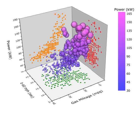
3D Graphs in Origin

› documents › excelHow to display text labels in the X-axis of scatter chart in ... Display text labels in X-axis of scatter chart. Actually, there is no way that can display text labels in the X-axis of scatter chart in Excel, but we can create a line chart and make it look like a scatter chart. 1. Select the data you use, and click Insert > Insert Line & Area Chart > Line with Markers to select a line chart. See screenshot:

Share :